
Now we’re not talking about the big broccoli plants that line the forests. We’re talking about a recursive data structure called the tree. These trees don’t provide Oxygen, but they do have branches. In this lesson, we’ll cover what exactly a tree is, discuss some of its properties, and chat about some of its applications. In particular, we’re going to focus on the binary search tree. As always, we’ll run through a basic implementation and share its performance. Let’s get started!
Table of Contents
What is a Tree?
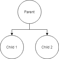
A tree is a recursive data structure constructed from nodes much like all of the linked list related data structures we’ve discussed before. However, the difference here is that each node can point to multiple other nodes. The catch is that trees must not contain any cycles. In other words, nodes must have only one parent (a parent being a node that points to a child). Also, nodes can’t reference themselves. In either case, we would end up with a different data structure called a graph.
We can imagine a tree pretty easily since we use them everyday. In fact, our file systems use a tree format for directories. While there are ways to introduce cycles with tools like symbolic and hard links, directories by default maintain the single parent rule for nodes. For example, Windows PCs usually have a drive named by some letter as the root (C://). This directory contains several directories which we typically call children. Each of those directories can have children as well and so on.
Properties of Trees
Trees by themselves are abstract data types meaning that they don’t really have any properties beyond what we’ve discussed above. A tree is really just a family of data structures that share the same fundamental rules. If we really want to get into the details, we’ll have to define some concrete data structures:
- Binary Trees
- Binary Search Trees
- AVL Trees
- Red-Black Trees
- Splay Trees
- N-ary Trees
- Trie Trees
- Suffix Trees
- Huffman Trees
- Heaps
- B-Trees
Credit for this list goes to Mr. Chatterjee from Quora.
For the purposes of this tutorial, we’ll focus on binary search trees. But wait! We’ll need to understand what a binary tree is first. A binary tree is a tree where each parent can have up to two children. This makes semantics pretty simple since we can refer to the children as left and right. Beyond that, binary trees don’t really have an special properties. In fact, they’re still a bit too abstract. Fortunately, binary search trees narrow down the scope a bit to make the data structure practical.
A binary search tree is one of many variations on the simple binary tree structure. In a binary search tree, we further restrict where data can be stored. In particular, we give nodes weights then use those weights to decide where new nodes get stored. For example, imagine that we had a tree with a root node of weight 15. If we bring along a node that has weight 7, where should we store it? Left or right?
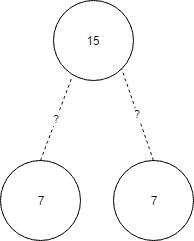
Obviously, we need to lay down some rules. On a binary search tree, the left side of a node is reserved for smaller values while it’s right side is reserved for larger values. In this case, we’ll send 7 to the left side.

Now just to complicate things a bit, what happens if a node comes along with a weight of 9? We’ll need to do a bit of traversal. In other words, we know that 9 is less than 15, so we’ll try to place the 9 where we just placed the 7. However, it turns out there’s a node already there, so what do we do? We simply start the process over while treating 7 as the new parent. Since 9 is greater than 7, we’ll place the new node to the right of 7.
Now this structure has some pretty interesting properties. It’s sort of like a sorted array, but we get the advantage of sped up inserts and deletes. It’s a best of both words type of data structure, but it still has some drawbacks. As we’ll see later, worst case performance across the board is O(N). This worst case scenario only occurs if the binary search tree is really just a linked list in disguise. Otherwise, we’re usually living a pretty happy O(log(N)).
As we can see above, there are several other types of trees that have different properties. Probably a good place to start would be the red-black tree. It’s a variation on the regular binary search tree which adds an additional constraint: the tree must stay balanced. From there, it might be appropriate to start exploring other types of trees. Maybe we can go over some of these types of trees in an advanced data structures series.
Applications of Trees
Trees in general have all sorts of purposes. However, since we only covered binary search trees, we’ll start there. The primary use of a binary search tree is for just that – search. In applications where we might be moving data in and out frequently, a binary search tree makes a great choice.
Trees also have loads of other important applications like path finding, compression algorithms, cryptography, and compilers. As we can see, studying data structures starts to open up doors into much more interesting computer science topics. That’s why it’s important to have strong fundamentals. They form the basis for just about every topic we might want to explore.
Java Tree Syntax
To create a tree, we’ll need to rework our old node class a bit. In particular, we’ll have to change that next pointer to a set of pointers. However, since we’ve spent all this time talking about binary search trees, we might as well go ahead and implement one. That means our new node class needs to support two pointers rather than one. Let’s call these pointers left and right.
public class Node {
  private int payload;
  private Node left;
  private Node right;

  // Implicit getters/setters/constructors
}
Great! Now that we have a new Node class, we can define the binary search tree class.
Class Definition
A basic tree should at least support the following functionality: insert, delete, search, and traverse. In addition, trees should also support the rotate functionality which changes the structure of the tree without changing the ordering. We won’t touch rotation for now, but we will handle everything else. For now, let’s implement a basic class.
public class BinarySearchTree {
  private Node root;

  // Implicit getters/setters/constructors
}
And that’s it! A tree is pretty simple. We just need a reference to the root, and we’re ready to start storing data. The magic happens during insertion. That’s where we’ll implement our logic to determine what type of tree we have.
Insertion
Since we’re implementing a binary search tree, we’ll need our insertion to properly navigate down the tree. To do so, we could use a loop. However, this can get pretty tricky since we don’t exactly know the depth of the tree at any given time. Instead, we’re going to use recursion. After all, trees are a family of recursive data structures.
public Node insert(Node root, int payload) {
  if (root == null) {
    root = new Node(payload);
  } else if (payload < root.getPayload()) {
    root.setLeft(insert(root.getLeft(), payload));
  } else if (payload > root.getPayload()) {
    root.setRight(insert(root.getRight(), payload));
  }
  return root;
}
Basically, the way this works is we first check if the root is null. If it is, we are starting our tree from scratch. If not, we check if the new node is going to go on the left or right side of the root. Regardless of the side, we then make a recursive call to the insert method again. However, this time we change the root. This process continues until we hit our base case which is a root that is null.
We can imagine this works because at any given moment we’re only dealing with a maximum of three nodes. These three nodes form a miniature tree with a single parent and two children. We’ll keep traversing down until we hit an empty child. At that point, we assign the child to its parent and traverse back up the tree. By the end, we’ll return the root of the tree which now contains the new node.
Deletion
Deletion is a bit more tricky because we may have to pull some nodes up. The following code snippet should do just that.
public Node delete(Node root, int payload) {
  if (root == null) {
    throw new NoSuchElementException("Element does not exist");
  } else if (payload < root.getPayload()) {
    root.setLeft(delete(root.getLeft(), payload));
  } else if (payload > root.getPayload()) {
    root.setRight(delete(root.getRight(), payload));
  } else {
    if (root.getLeft() == null) {
      root = root.getRight();
    } else if (root.getRight() == null) {
      root = root.getLeft();
    } else {
      tempNode = root.getLeft();
      while(tempNode.getRight() != null) {
        tempNode = tempNode.getRight();
      }
      root.setPayload(tempNode.getPayload);
      root.setLeft(delete(root.getLeft(), tempNode.getPayload()));
    }
  }
  return root;
}
As we can see, delete operates almost exactly the same as insert. We simply traverse down the tree until we find the node we require. However, there’s a new special case that occurs once we find it. Basically, we just check if there is a left node. If not, we pull up the right node and call it a day. Likewise, if there’s no right node, we pull up the left node.
Unfortunately, the decision isn’t always that easy. If both the left and right nodes exist, we need a way to fill in the node we just deleted. To do so, we actually pull up the rightmost node on the left side. Yeah, that does sound confusing, but basically we just want the largest node on the left side. That way we can confirm everything is still organized.
Once we’ve grabbed the greatest node on the left subtree, we store its payload in our current root. Then we delete that node. To do so, we actually make another recursive call to delete. This will eventually filter down and catch the case where both children are null. In which case, we just set it to null.
Search
Now that we understand insertion and deletion, search should be a joke. With search we have two base cases: root is null or root equals the value we’re trying to find.
public boolean search(Node root, int payload) {
  if (root == null) {
    return false;
  } else if (root.getPayload() == payload) {
    return true;
  } else if (payload < root.getPayload()) {
    return search(root.getLeft());
  } else {
    return search(root.getRight());
  }
}
That should be all we need to run a quick search. Typically, we would want to avoid this many return statements, but in this case the method is simple enough.
Traversal
Okay, so it probably seems like we’re done with trees. However, we’re not quite finished. We need to touch on a subject called traversal for a moment. The reason being that sometimes we need to make sure we’ve visited every node once. This is a concept that we’ll definitely need to get familiar with before we start talking about graphs.
On lists, this wasn’t really an issue. We can simply run from beginning to end to complete a traversal. On a tree, however, we have options: in-order, pre-order, and post-order. These three different traversals have different purposes but ultimately accomplish the same goal: visit every node in a tree exactly once.
The purpose of in-order traversal is to provide a linear copy of the data in the tree. For a binary search tree, that means creating a sorted list from all the data in the tree. Pre-order traversal is typically used to clone a tree, but it’s also used to produce prefix expression from an expression tree. Finally, Post-order is used for deleting trees, but it can also be used to generate a postfix expression from an expression tree. The following details the node traversal order for each of these methods of traversal:
- In-order: left, root, right
- Pre-order: root, left, right
- Post-order: left, right, root
While there are other traversal strategies, these are the fundamental ones. We should get pretty familiar with them.
Summary
As stated several times already, trees don’t have any inherent properties for the sake of performance. As a result, the following table only details the performance of binary search trees.
| Algorithm | Running Time |
|---|---|
| Access | O(N) |
| Insert | O(N) |
| Delete | O(N) |
| Search | O(N) |
Keep in mind that all the tables in this series assume worst case. A binary search tree is only worst case when it degenerates to a linked lists. In other words, we get a chain of left nodes without right nodes or vice versa.
As always, thanks for taking the time to check The Renegade Coder out today. Hopefully, you learned something!
Recent Posts
Suppose someone says, "AI has problems, but it's fine as long as a human reviews the output." Do we really think that's the way forward? I sure don't.
As a self-identified AI hater, r/vibecoding should be the last place I visit, but here we are.